Random projection

Random projection is a dimensionality reduction technique that projects high-dimensional data onto a lower-dimensional subspace using a random matrix. It’s based on the Johnson-Lindenstrauss lemma, which states that distances between points are approximately preserved when projected to a sufficiently high dimensional random subspace.

The computational demands of evaluating the full expected site frequency spectrum (SFS) increase substantially with both sample size and model complexity. We implement random projection as an efficient, low-dimensional approximation method that preserves essential signals of the full SFS while dramatically reducing computational cost.

Please refer to momi3 Tutorial first before exploring random projections. All random projection capabilities are seamlessly integrated into demestats’s core architecture, accessible through the same functional interfaces demonstrated in the momi3 Tutorial documentation. Users can use these accelerated methods by simply providing an additional parameter to existing functions, maintaining the same intuitive workflow while gaining significant performance benefits.

The corresponding Jupyter notebook is available at docs/tutorial_code/random_projection.ipynb.

Let us revisit the isolation-with-migration (IWM) model:

import msprime as msp
import demesdraw

demo = msp.Demography()
demo.add_population(initial_size=5000, name="anc")
demo.add_population(initial_size=5000, name="P0")
demo.add_population(initial_size=5000, name="P1")
demo.set_symmetric_migration_rate(populations=("P0", "P1"), rate=0.0001)
demo.add_population_split(time=1000, derived=["P0", "P1"], ancestral="anc")
g = deme.to_demes()
demesdraw.tubes(g)

sample_size = 10 # simulate 10 diploids
samples = {"P0": sample_size, "P1": sample_size}
ts = msp.sim_mutations(
    msp.sim_ancestry(
        samples=samples, demography=demo,
        recombination_rate=1e-8, sequence_length=1e8, random_seed=12
    ),
    rate=1e-8, random_seed=13
)

# Each population will have 20 haploids
afs_samples = {"P0": sample_size * 2, "P1": sample_size * 2}
afs = ts.allele_frequency_spectrum(
    sample_sets=[ts.samples([1]), ts.samples([2])],
    span_normalise=False,
    polarised = True
)

The first step is to create the random projections using prepare_projection and one must provide the sample configuration (afs_samples), the observed frequency spectrum (afs), the number of projections to use and a seed for reproducibility.

sequence_length = None
num_projections = 200
seed = 50 

proj_dict, einsum_str, input_arrays = prepare_projection(afs, afs_samples, sequence_length, num_projections, seed)

The function returns three components that collectively enable efficient likelihood computation via random projection: proj_dict contains the random projection vectors, einsum_str is a string specifying the Einstein summation for tensor operations, and input_arrays are preprocessed arrays that serve as inputs to the jax.numpy.einsum call, optimized for JAX’s just-in-time compilation. Together, these components are used for computing the projected likelihood with optimal computational efficiency within JAX’s differentiable programming framework.

To obtain a low dimensional representation of the SFS, we use tensor_prod which takes in a dictionary of the random projections and applies them to the full expected SFS evaluated at the specified parameter values in the paths variable. We follow the same setup in momi3 Tutorial documentation and create an ExpectedSFS object to apply tensor_prod.

paths = {frozenset({('demes', 0, 'epochs', 0, 'end_size'),
        ('demes', 0, 'epochs', 0, 'start_size')}):3000.,
    frozenset({('demes', 1, 'epochs', 0, 'end_size'),
        ('demes', 1, 'epochs', 0, 'start_size')}): 6000.,
    frozenset({('demes', 2, 'epochs', 0, 'end_size'),
        ('demes', 2, 'epochs', 0, 'start_size')}): 4000.}

esfs_obj = ExpectedSFS(g, num_samples=afs_samples)
lowdim_esfs = esfs_obj.tensor_prod(proj_dict, paths)

Projected SFS log-likelihood

Each projection summarizes the full SFS with a single number, so the dimension of lowdim_esfs will match the number of projections used. One can also easily compute the likelihood using projection_sfs_loglik. The likelihood follows similar principals as sfs_loglik where BOTH a sequence length and mutation rate (theta) must be provided to indicate Poisson likelihood.

To use the multionmial likelihood:

from demestats.loglik.sfs_loglik import projection_sfs_loglik

mult_ll = projection_sfs_loglik(esfs_obj, paths, proj_dict, einsum_str, input_arrays)

To use the Poisson likelihood, one must provide both the sequence length and mutation rate (theta):

pois_ll = projection_sfs_loglik(esfs_obj, paths, proj_dict, einsum_str, input_arrays, sequence_length=1e-8, theta=1e-8)

Differentiable log-likelihood

Using JAX’s automatic differentiation capabilities via the jax.value_and_grad, one can compute the gradient and log-likelihood at specific parameter settings. Here we show an example of computing the gradient with respect to the rate of migration from P0 to P1 at 0.0002.

import jax
param_key = frozenset({('migrations', 0, 'rate')})

@jax.value_and_grad
def ll_at(val):
    params = {param_key: val}
    return projection_sfs_loglik(esfs_obj, params, proj_dict, einsum_str, input_arrays, sequence_length=None, theta=None)

val = 0.0002
loglik_value, loglik_grad = ll_at(val)
# Provide both a sequence length and mutation rate to use poisson likelihood

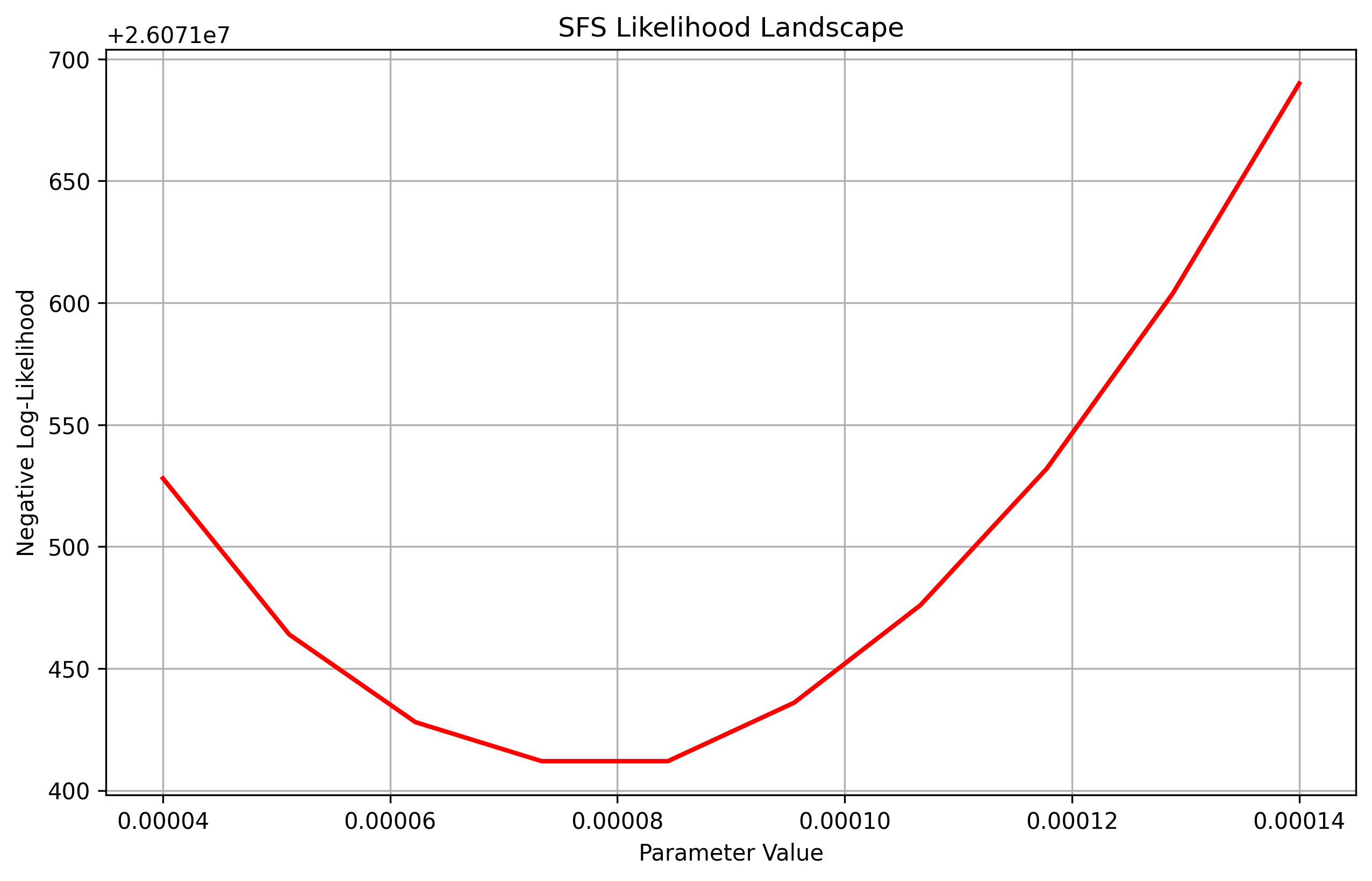
Log-likelihood Visualization

To visualize the log-likelihood over one parameter using random projections, using plot_sfs_likelihood function we can pass in an argument for projection and num_projections.

import jax.numpy as jnp
from demestats.plotting_util import plot_sfs_contour

# override the parameter of interest
paths = {
    frozenset({("migrations", 0, "rate")}): 0.0001,
}

vec_values = jnp.linspace(0.00004, 0.00014, 10)
result = plot_sfs_likelihood(demo.to_demes(), paths, vec_values, afs, afs_samples, num_projections=200, seed=5, projection=True)

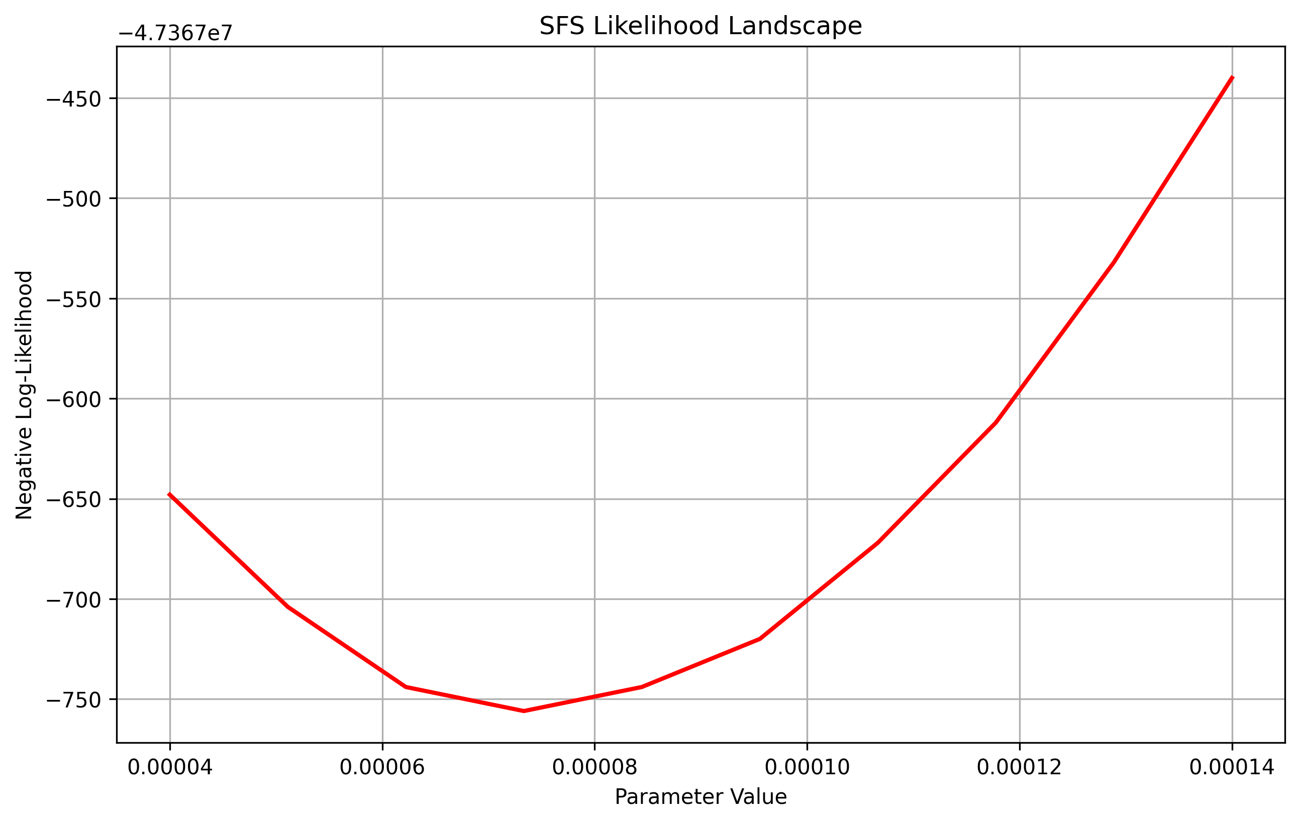
If one wanted to visualize the Poisson log-likelihood we just pass in sequence length and mutation rate.

paths = {
frozenset({("migrations", 0, "rate")}): 0.0001,
}

vec_values = jnp.linspace(0.00004, 0.00014, 10)
sequence_length = 1e8
theta = 1e-8
result = plot_sfs_likelihood(demo.to_demes(), paths, vec_values, afs, afs_samples, num_projections=200, seed=5, projection=True, sequence_length=sequence_length, theta=theta)

Similarily if one wanted to plot contour plots for visualizing two variables at once, we use the same plot_sfs_contour and pass in an argument projection.

from demestats.plotting_util import plot_sfs_contour

paths = {
    frozenset({
        ("demes", 1, "epochs", 0, "end_size"),
        ("demes", 1, "epochs", 0, "start_size"),
    }): 4000.,
    frozenset({
        ("demes", 2, "epochs", 0, "end_size"),
        ("demes", 2, "epochs", 0, "start_size"),
    }): 4000.,
}

param1_vals = jnp.linspace(4000, 6000, 10)
param2_vals = jnp.linspace(4000, 6000, 10)

result = plot_sfs_contour(demo.to_demes(), paths, param1_vals, param2_vals, afs, afs_samples, projection=True, num_projections=200, seed=5)

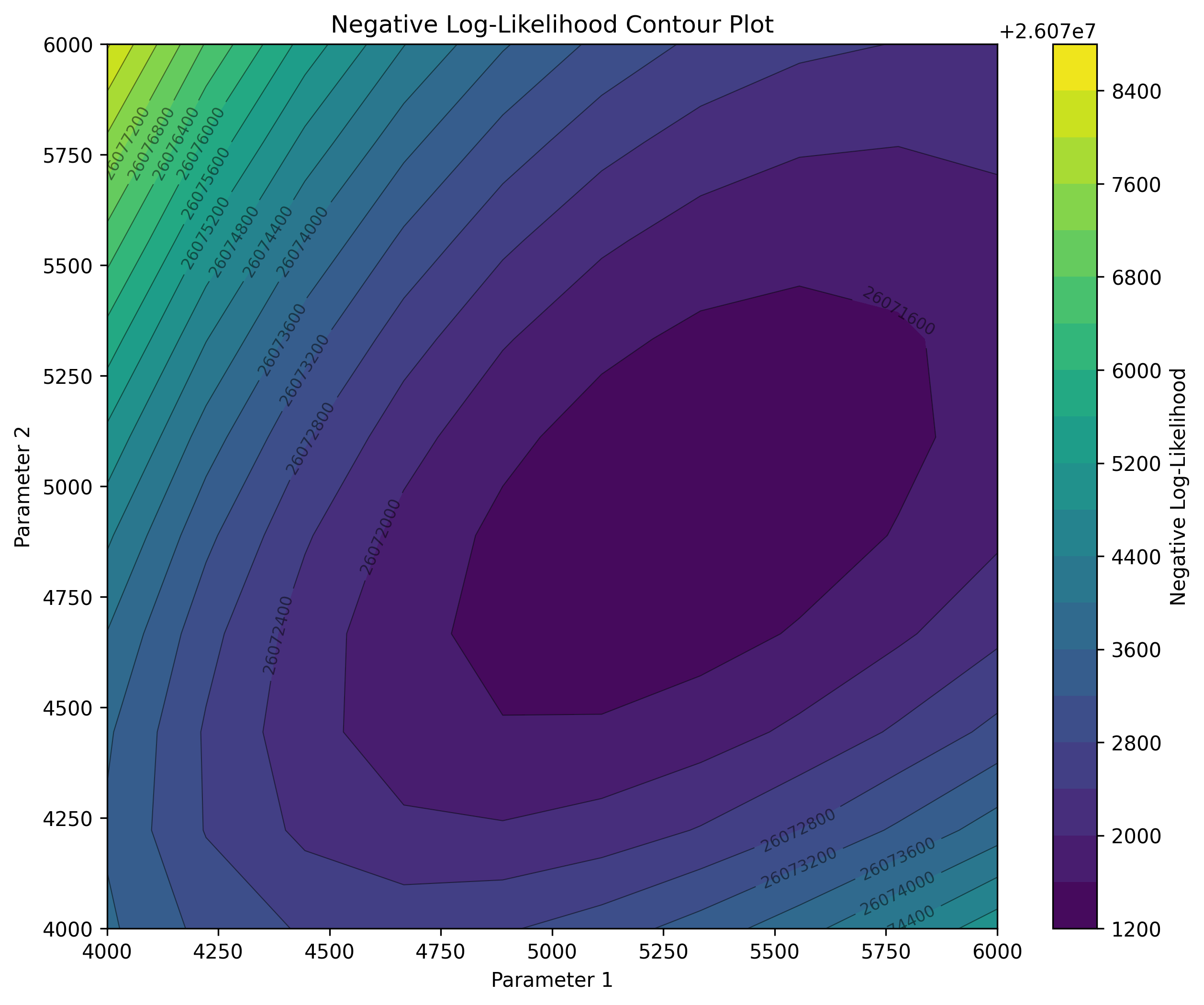
These examples highlight that the projected SFS can capture similar signals as the full expected SFS, please refer to the preprint for further details.