momi3 Tutorial (within demestats)
This tutorial is a self-contained introduction to momi3, implemented as part of the
demestats package (specifically the demestats.sfs modules). demestats also includes
other components (ICR/CCR curves, event trees, constraints, etc.), but this guide focuses
only on the SFS-based inference workflow that people refer to as momi3.
The corresponding Jupyter notebook is available at docs/tutorial_code/momi3_tutorial.ipynb.
Overview
The momi3 workflow inside demestats consists of:
Simulating (or loading) genetic data.
Computing an allele-frequency spectrum (AFS).
Building an
ExpectedSFSmodel from ademes.Graph.Evaluating SFS log-likelihoods.
(Optionally) optimizing demographic parameters with constraints.
Simulation
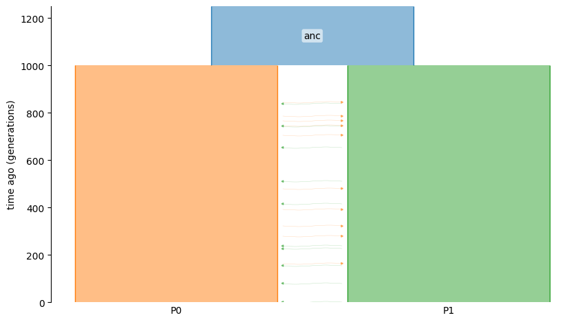
We will simulate a simple isolation-with-migration (IWM) model with two populations.
This uses msprime to build a demography and simulate ancestry/mutations.
import msprime as msp
import demesdraw

demo = msp.Demography()
demo.add_population(initial_size=5000, name="anc")
demo.add_population(initial_size=5000, name="P0")
demo.add_population(initial_size=5000, name="P1")
demo.set_symmetric_migration_rate(populations=("P0", "P1"), rate=0.0001)
demo.add_population_split(time=1000, derived=["P0", "P1"], ancestral="anc")

g = demo.to_demes() # this demes.Graph g will be the input to demestats
demesdraw.tubes(g)
Simulate ancestry and mutations, with 10 diploids from each population:
sample_size = 10
samples = {"P0": sample_size, "P1": sample_size}

anc = msp.sim_ancestry(
    samples=samples,
    demography=demo,
    recombination_rate=1e-8,
    sequence_length=1e8,
    random_seed=12,
)

ts = msp.sim_mutations(anc, rate=1e-8, random_seed=13)
Compute the AFS (allele-frequency spectrum):
# afs_samples is based on the number of haploids
afs_samples = {"P0": sample_size * 2, "P1": sample_size * 2}
afs = ts.allele_frequency_spectrum(
    sample_sets=[ts.samples([1]), ts.samples([2])],
    span_normalise=False,
    polarised=True,
)
For more details regarding simulation, please refer to msprime.
ExpectedSFS (momi3 core)
The ExpectedSFS object is the core momi3 component. It maps a demes.Graph and sample
configuration to the expected spectrum under a demographic model. We will use all of the simulated data, otherwise one can edit afs_samples to change the sample configuration.
from demestats.sfs import ExpectedSFS

esfs = ExpectedSFS(g, num_samples=afs_samples)
expected = esfs(params={})
Note that passing in params={} evaluates the expected spectrum under the constructed demographic model g.
Parameter overrides
To override and evaluate the model at specific parameter settings:
from demestats.event_tree import EventTree

et = EventTree(g)

# Pick variables (by path) from the event tree.
v_split = et.variable_for(("demes", 0, "epochs", 0, "end_time"))
v_mig = et.variable_for(("migrations", 0, "rate"))

# All other non-selected parameters will use the values specified by model g.
# Construct new parameter setting
params = {
    v_split: 1200.0,
    v_mig: 2e-4,
}
The params dict can then be passed into ExpectedSFS:
esfs = ExpectedSFS(g, num_samples={"P0": 20, "P1": 20})
expected = esfs(params=params)
SFS log-likelihood
For likelihood-based inference, use the SFS log-likelihood helper from
demestats.loglik.sfs_loglik.
To compute the multionmial likelihood:
from demestats.loglik.sfs_loglik import sfs_loglik

mult_ll = sfs_loglik(
    afs=afs,
    esfs=expected,
)
To use the Poisson likelihood, one must provide both the sequence length and mutation rate (theta):
pois_ll = sfs_loglik(
    afs=afs,
    esfs=expected,
    sequence_length=1e8,
    theta=1e-8,
)
Differentiable log-likelihood
Using JAX’s automatic differentiation capabilities via jax.value_and_grad, one can compute the gradient and log-likelihood given the expected and observed SFS. Here we
show an example of computing the gradient with respect to the rate of migration from P0 to P1 at 0.0002.
import jax
param_key = frozenset({('migrations', 0, 'rate')})

@jax.value_and_grad
def ll_at(val):
    params = {param_key: val}
    esfs = esfs_obj(params)
    return sfs_loglik(afs, esfs, 1e8, 1e-8)

val = 0.0002
loglik_value, loglik_grad = ll_at(val)
# To compute gradient of multinomial likelihood, simply omit sequence_length and theta
Parameterization and constraints
demestats automatically generates parameter constraints for a given model via
EventTree and constraints_for. This is part of the momi3 workflow because it defines
the feasible parameter space for SFS-based optimization.
from demestats.constr import EventTree, constraints_for

et = EventTree(g)
variables = et.variables

cons = constraints_for(et, *variables)
A_eq, b_eq = cons["eq"]
A_ineq, b_ineq = cons["ineq"]
Please refer to Model Constraints to understand how to modify the constraints to one’s needs.
Putting it together (minimal optimization sketch)
A full optimizer is not shown here, but the typical flow is:
Create a vector for the parameters of interest (subset of
et.variables).Use
constraints_forto get linear constraints.Construct
ExpectedSFSobject and obtain the expected spectrum.Evaluate SFS log-likelihood and optimize.
If you want a complete optimization example, use the notebook at
docs/tutorial_code/momi3_optimization.ipynb and refer to SFS Optimization.
Where to go next
To compute approximations of the full expected SFS, please see
Random ProjectionFor other
demestatsfeatures (ICR/CCR curves, event trees, etc.), see the main documentation sectionsICRandCCR.For API details, see the generated module reference under
API.