SFS Optimization

This page demonstrates a constrained optimization workflow with demestats. It stands on its own, separate from the main tutorial.

This tutorial shows how to create a customizable SciPy optimizer for any demographic model using scipy.minimize. It is not a primer on numerical optimization. SciPy’s API/behaviour can change across versions — We are not responsible for any updates/errors made to scipy.minimize.

You can find the code in docs/tutorial_code/momi3_optimization.ipynb.

Imports

import numpy as np
import jax
import jax.numpy as jnp
import msprime as msp
from scipy.optimize import Bounds, LinearConstraint, minimize
from demestats.fit.util import _dict_to_vec, _vec_to_dict_jax, _vec_to_dict, create_inequalities, make_whitening_from_hessian, pullback_objective, create_constraints
from typing import Any, List, Mapping, Set, Tuple
from demestats.sfs import ExpectedSFS
from demestats.constr import EventTree, constraints_for
from demestats.fit.fit_sfs import _compute_sfs_likelihood, neg_loglik

Path = Tuple[Any, ...]
Var = Path | Set[Path]
Params = Mapping[Var, float]

Revisiting the IWM model

demo = msp.Demography()
demo.add_population(initial_size=5000, name="anc")
demo.add_population(initial_size=5000, name="P0")
demo.add_population(initial_size=5000, name="P1")
demo.set_symmetric_migration_rate(populations=("P0", "P1"), rate=0.0001)
demo.add_population_split(time=1000, derived=["P0", "P1"], ancestral="anc")

sample_size = 10 # we simulate 10 diploids
samples = {"P0": sample_size, "P1": sample_size}
ts = msp.sim_mutations(
    msp.sim_ancestry(
        samples=samples, demography=demo,
        recombination_rate=1e-8, sequence_length=1e8, random_seed=12
    ),
    rate=1e-8, random_seed=13
)

# For each population, use 20 haploids for the AFS
afs_samples = {"P0": sample_size * 2, "P1": sample_size * 2}
afs = ts.allele_frequency_spectrum(
    sample_sets=[ts.samples([1]), ts.samples([2])],
    span_normalise=False,
    polarised=True
)

Inspecting and selecting parameters to optimize

Inspect the parameters you can work with:

et = EventTree(demo.to_demes())
et.variables

Suppose now we wish to optimize the following parameters, their associated values will be the initial guesses in the optimization process. We collect those parameters into a dictionary:

paths = {frozenset({('demes', 0, 'epochs', 0, 'end_size'),
        ('demes', 0, 'epochs', 0, 'start_size')}):3000.,
        frozenset({('demes', 1, 'epochs', 0, 'end_size'),
            ('demes', 1, 'epochs', 0, 'start_size')}): 6000.,
        frozenset({('demes', 2, 'epochs', 0, 'end_size'),
            ('demes', 2, 'epochs', 0, 'start_size')}): 4000.}

cons = create_constraints(demo.to_demes(), paths)

The create_constraints function is a helper function that takes in a dictionary of parameters and calls on constraints_for to output the associated constraints. For any contrained optimization method, one needs a set of parameters they wish to optimize, the constraints, a way to compute the expected SFS, and a way to compute the likelihood and its gradient.

Initial required setup

###### Part 1 #####
path_order: List[Var] = list(paths) # convert parameters into list
x0 = jnp.array(_dict_to_vec(paths, path_order)) # convert initial values into a vector
lb = jnp.array([0, 0, 0])
ub = jnp.array([1e8, 1e8, 1e8])
afs = jnp.array(afs)
# create ExpectedSFS object
esfs = ExpectedSFS(demo.to_demes(), num_samples=afs_samples)

###### Part 2 #####
seed = 5
projection = False
sequence_length = None
theta = None

# This if statements creates the random projection vector
# Please refer to Random Projection documentation
if projection:
    proj_dict, einsum_str, input_arrays = prepare_projection(afs, afs_samples, sequence_length, num_projections, seed)
else:
    proj_dict, einsum_str, input_arrays = None, None, None

##### Part 3 ######
args_nonstatic = (path_order, proj_dict, input_arrays, sequence_length, theta, projection, afs)
args_static = (esfs, einsum_str)
L, LinvT = make_whitening_from_hessian(_compute_sfs_likelihood, x0, args_nonstatic, args_static)
preconditioner_nonstatic = (x0, LinvT)
g = pullback_objective(_compute_sfs_likelihood, args_static)
y0 = np.zeros_like(x0)

lb_tr = L.T @ (lb - x0)
ub_tr = L.T @ (ub - x0)

For scipy.minimize, the setup requires three parts. Construction of likelihood functions are described at the end of the tutorial.

Part 1

• While dictionary representations provide intuitive tracking of parameter states, most numerical optimizers require vectorized inputs. To address this, parameter dictionaries must be transformed into compatible vector formats.

• Based on our benchmarking with scipy.minimize, we recommend explicitly defining lower (lb) and upper (ub) bounds to constrain the search space, which significantly improves optimization performance and stability.

Part 2

One must make two decisions:

• First decision is to specify a boolean projection to indicate whether we will be using the random projection as an approximation of the expected SFS. Here projection = False indicates we do not use random projections and instead calculate the expected SFS exactly.

• Second decision is the type of likelihood to use, one must specify BOTH sequence_length and theta to use the Poisson likelihood, otherwise leave both as None to use the Multinomial likelihood.

Part 3

This setup is optional and will depend on the user’s preference. In our experience with scipy.minimize, due to the magnitude difference between parameters such as the migration rate and population sizes, the gradient with respect to each variable will cause parameter updates to be unstable. We implemented a preconditioning method that makes our problem more suitable for optimization. Instead of optimizing over the classical likelihood function _compute_sfs_likelihood, we transform the likelihood function and the bounds to instead optimize over a function g with better conditioning. For more information on preconditioning.

Constraints and scipy.optimize.LinearConstraint

Use constraints_for to derive the linear constraints for your chosen parameters. It returns a dict with:

• "eq" → (Aeq, beq) for equality constraints

• "ineq" → (G, h) for inequalities.

These map directly to SciPy’s scipy.optimize.LinearConstraint:

linear_constraints: list[LinearConstraint] = []

Aeq, beq = cons["eq"]
A_tilde = Aeq @ LinvT
b_tilde = beq - Aeq@x0
if Aeq.size:
    linear_constraints.append(LinearConstraint(A_tilde, b_tilde, b_tilde))

G, h = cons["ineq"]
if G.size:
    linear_constraints.append(create_inequalities(G, h, LinvT, x0, size=len(paths)))

As explained in the Model Constraints, one would use create_inequalities to modify the output of constraints_for into the appropriate scipy.optimize.LinearConstraint format.

Create and run the optimizer

The final step is use an optimizer. Here we use scipy.minimize with constrained optimizer "trust-constr". Please refer to scipy.minimize

gtol = 1e-5
xtol = 1e-5
maxiter = 1000
barrier_tol = 1e-5

res = minimize(
    fun=neg_loglik,
    x0=y0,
    jac=True,
    args = (g, preconditioner_nonstatic, args_nonstatic, lb_tr, ub_tr),
    method=method,
    constraints=linear_constraints,
    options={
        'gtol': gtol,
        'xtol': xtol, 
        'maxiter': maxiter,
        'barrier_tol': barrier_tol,
    }
)

x_opt = np.array(x0) + LinvT @ res.x

Due to preconditioning, we must transform the variable to inspect our final estimates:

print("Optimal parameters: ", _vec_to_dict(jnp.asarray(res.x), path_order))
print("\nFinal likelihood evaluation: ", res.fun)
print("Optimal parameters as a vector: ", x_opt)

For the simulated example, the estimates are close to the true values:

Optimal parameters:  
{frozenset({('demes', 0, 'epochs', 0, 'end_size'), ('demes', 0, 'epochs', 0, 'start_size')}): 5016.814453125, 

frozenset({('demes', 1, 'epochs', 0, 'start_size'), ('demes', 1, 'epochs', 0, 'end_size')}): 5238.4287109375, 

frozenset({('demes', 2, 'epochs', 0, 'start_size'), ('demes', 2, 'epochs', 0, 'end_size')}): 5025.2666015625}
    
Final negative log-likelihood evaluation:  430751.8125
Optimal parameters as a vector:  [5016.8145 5238.4287 5025.2666]

We have this full pipeline described above wrapped in a single fit_sfs function for convenience. See the API documentation for available options and implementation details. The convenience of demestats is that each component of the optimization pipeline can be modified and operated on its own, but if one wants to use the fit_sfs function:

from demestats.fit.fit_sfs import fit

optimal_params, final_loglikelihood, optimal_params_vector = fit(demo.to_demes(), paths, afs, afs_samples, cons, lb, ub)

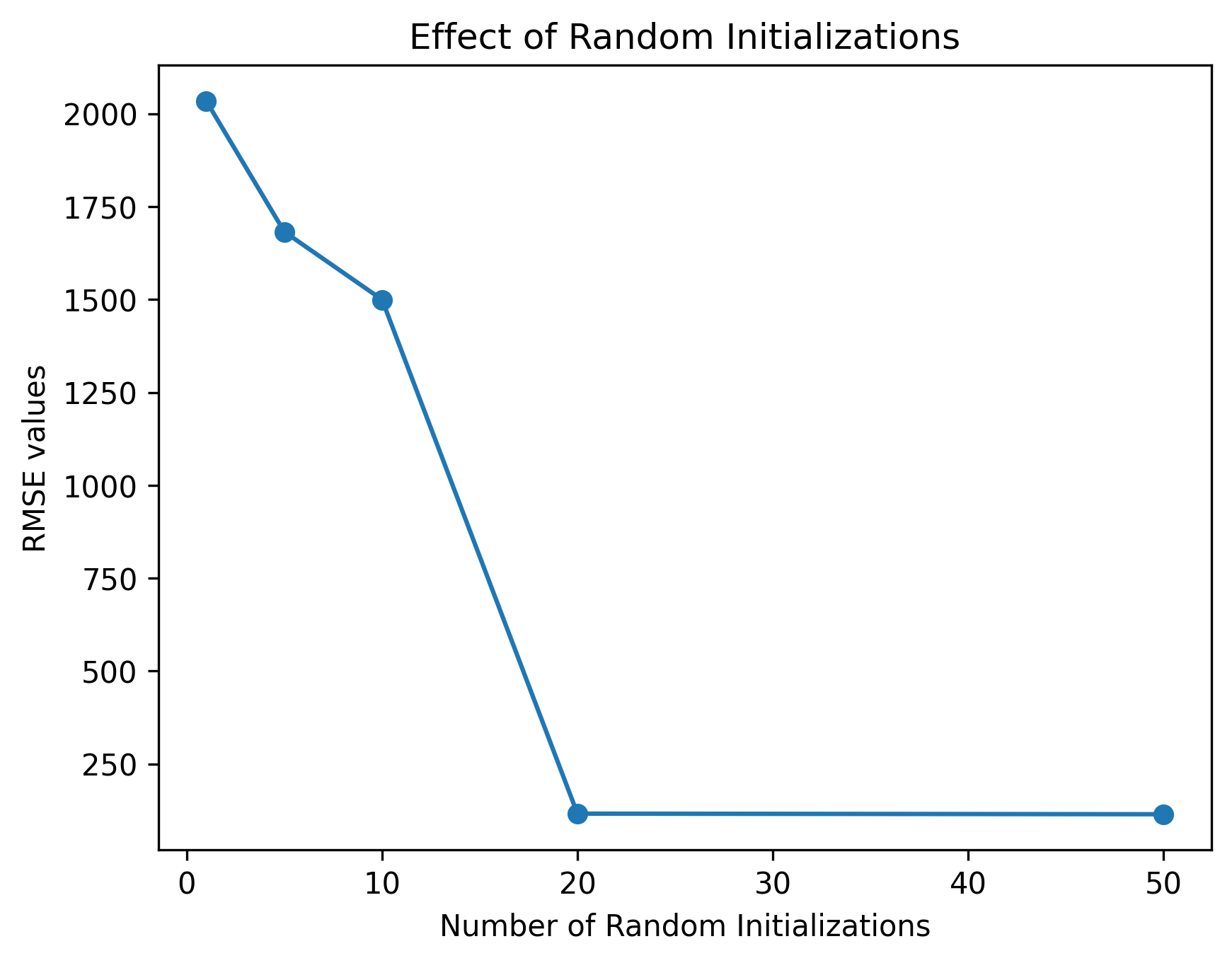
Importance of Random Initial Starting Points

Due to the possible non-convex nature of the likelihood function, proper optimization requires initializing many random starting points and selecting the run that achieves the optimal likelihood. The figure below illustrates how poorly chosen initial points can lead to local minimums.

Understanding the objective function

Below is just an example of the objective function we designed for scipy.minimize to give users a better understanding of creating an inference pipeline.

def _compute_sfs_likelihood(vec, args_nonstatic, args_static):
    (path_order, proj_dict, input_arrays, sequence_length, theta, projection, afs) = args_nonstatic
    (esfs_obj, einsum_str) = args_static
    params = _vec_to_dict_jax(vec, path_order)
    
    if projection:
        loss = -projection_sfs_loglik(esfs_obj, params, proj_dict, einsum_str, input_arrays, sequence_length, theta)
        return loss
    else:
        esfs = esfs_obj(params)
        loss = -sfs_loglik(afs, esfs, sequence_length, theta)
        return loss

def neg_loglik(vec, g, preconditioner_nonstatic, args_nonstatic, lb, ub):
    if jnp.any(vec >= ub):
        return jnp.inf, jnp.full_like(vec, 1e10)

    if jnp.any(vec <= lb):
        return jnp.inf, jnp.full_like(vec, -1e10)

    return g(vec, preconditioner_nonstatic, args_nonstatic)

The objective function one would typically use for scipy.minimize would look something like neg_loglik, where vec represents the parameter values, g computes the likelihood and gradient in a transformed space by indirectly calling _compute_sfs_likelihood, and the other variables are arguments necessary for computing the likelihood. To limit the parameter search space we define variables lb and ub. The _compute_sfs_likelihood function unpacks all of the arguments and makes a simple check for whether a user wants to compute the projected or full expected SFS.