Special Examples
Changing the grouping of paths within a frozenset
The corresponding Jupyter notebook is available at docs/tutorial_code/examples.ipynb.
Note that frozenset parameters cannot be directly removed, since they are derived from the demographic model structure. However, frozenset parameters disappear and change when the model no longer forces equality during its construction. For example, if a population’s size is not constant across an epoch (e.g., exponential growth), its start_size and end_size become separate variables instead of a single tied frozenset.
To show that, let’s define a new demographic model where population size changes over time.
import msprime as msp
import demesdraw
demo1 = msp.Demography()
demo1.add_population(name="anc", initial_size=5000)
demo1.add_population(name="P0", initial_size=5000, growth_rate=0.002)
demo1.add_population(name="P1", initial_size=5000, growth_rate=0.002)
demo1.set_symmetric_migration_rate(populations=("P0", "P1"), rate=0.0001)
demo1.add_population_split(time=1000, derived=[f"P{i}" for i in range(2)], ancestral="anc")
This is a model where P0 and P1 grow exponentially from an initial size of 5000 at a rate of 0.002 per generation. We examine the parameters and constraints:
from demestats.constr import EventTree
h = demo1.to_demes()
et = EventTree(h)
et.variables
We can see that in the output, the population sizes for P0 and P1 are now treated as separate parameters (no longer in a single frozenset), since they can differ due to exponential growth. The ancestral population size remains constant throughout time, so it is still grouped in a frozenset.
Correspondingly, the constraints will reflect this change. If you want to peek at all of the constraints, you can run:
from demestats.constr import constraints_for
constraints_for(et, *et.variables)
You would see that the start and end sizes for P0 and P1 are now independent variables without equality constraints or frozenset tying them together.
Population size change example
We now consider a more complex demographic model that includes population size changes and migration rate changes over time.
import numpy as np

# Create demography object
demo2 = msp.Demography()

# Add populations
demo2.add_population(initial_size=4000, name="anc")
demo2.add_population(initial_size=500, name="P0", growth_rate=-np.log(3000 / 500)/66)
demo2.add_population(initial_size=500, name="P1", growth_rate=-np.log(3000 / 500)/66)
demo2.add_population(initial_size=100, name="P2", growth_rate=-np.log(3000 / 100)/66)

# Set initial migration rate
demo2.set_symmetric_migration_rate(populations=("P0", "P1"), rate=0.0001)
demo2.set_symmetric_migration_rate(populations=("P1", "P2"), rate=0.0001)

# population size changes near 65–66 generations
demo2.add_population_parameters_change(
    time=65,
    initial_size=3000,  # Bottleneck: reduce to 1000 individuals
    population="P0",
    growth_rate=0
)
demo2.add_population_parameters_change(
    time=65,
    initial_size=3000,  # Bottleneck: reduce to 1000 individuals
    population="P1",
    growth_rate=0
)
demo2.add_population_parameters_change(
    time=66,
    initial_size=3000,  # Bottleneck: reduce to 1000 individuals
    population="P2",
    growth_rate=0
)

# Migration rate change changed to 0.001 AFTER 500 generation (going into the past)
demo2.add_migration_rate_change(
    time=66,
    rate=0.0005,
    source="P0",
    dest="P1"
)
demo2.add_migration_rate_change(
    time=66,
    rate=0.0005,
    source="P1",
    dest="P0"
)
demo2.add_migration_rate_change(
    time=66,
    rate=0.0005,
    source="P1",
    dest="P2"
)
demo2.add_migration_rate_change(
    time=66,
    rate=0.0005,
    source="P2",
    dest="P1"
)

# THEN add the older events (population split at 1000)
demo2.add_population_split(time=5000, derived=["P0", "P1", "P2"], ancestral="anc")

# Visualize the demography
p = demo2.to_demes()
demesdraw.tubes(p, log_time=True)
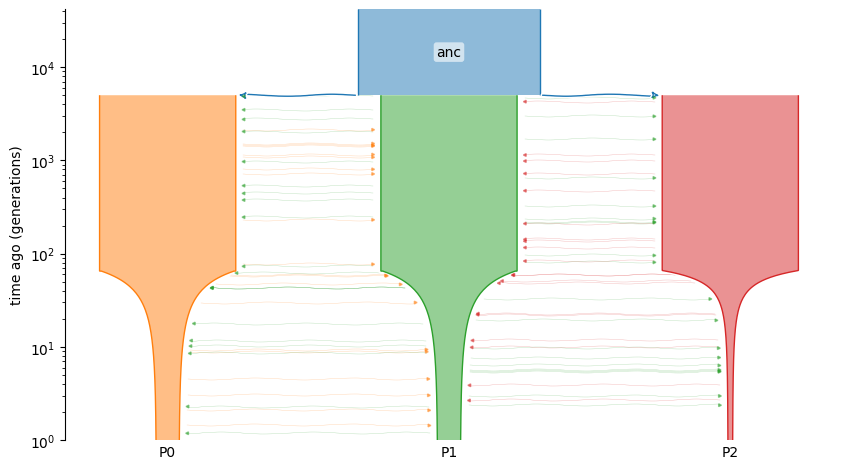
Note The choice to use 65 and 66 generations is intentional. In demestats, the event times that coincide exactly are treated as the same time identity and will be grouped into a single parameter (check the notation section for more details). That’s useful when events truly share a time, but it can also merge parameters you’d prefer to optimize independently. The only way to avoid having frozensets forcefully constrain parameters to be equal is to modify the construction of the model. Offsetting one set of events to 65 generations and the others to 66 keeps them as distinct time variables.
You can inspect the parameters/constraints and see the effect using the same commands as before:
et = EventTree(p)
print(et.variables)
print(constraints_for(et, *et.variables))
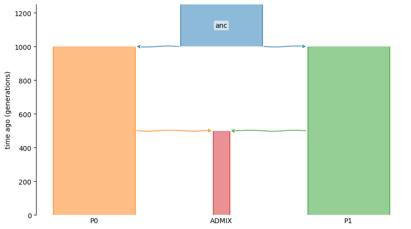
Admixture example
Another common demographic scenario of interest is admixture.
Here, we extend the simple IWM example to include four populations: one ancestral population (anc) and three contemporary populations (P0, P1, and ADMIX). We introduce an admixture event in which ADMIX is formed from P0 and P1 500 generations ago.
demography = msp.Demography()
demography.add_population(name="P0", initial_size=5000)
demography.add_population(name="P1", initial_size=5000)
demography.add_population(name="ADMIX", initial_size=1000)
demography.add_population(name="anc", initial_size=5000)
demography.add_admixture(
    time=500, derived="ADMIX", ancestral=["P0", "P1"], proportions=[0.4, 0.6])
demography.add_population_split(time=1000, derived=["P0", "P1"], ancestral="anc")

q = demography.to_demes()
demesdraw.tubes(q)