ICR Tutorial
This tutorial is an introduction to ICR, implemented as part of the
demestats package (specifically the demestats.icr modules). demestats also includes
other components (ICR/CCR curves, SFS, event trees, constraints, etc.), but this guide focuses
only on the ICR-based inference workflow.
The corresponding Jupyter notebook is available at docs/tutorial_code/icr_tutorial.ipynb.
Instantaneous Coalescent Rate (ICR)
This tutorial shows how to compute instantaneous coalescence rate
(ICR) curves for several total sample sizes k, using both the exact solver
and the mean-field approximation.
demestats.icr.ICRCurve: exact lineage-count CTMC. Accurate, but the state space grows quickly withk.demestats.icr.ICRMeanFieldCurve: deterministic mean-field approximation. Much faster for larger sample sizes.
demestats returns the coalescence hazard c(t) (also known as the ICR) together with the log-survival curve log_s(t).
Overview
The ICR workflow inside demestats consists of:
Simulating (or loading) tree sequence data.
Define sample size, timepoints, and sampling configuration.
Building an
ICRCurveorICRMeanFieldCurvemodel from ademes.Graph.Evaluating ICR log-likelihoods.
(Optionally) optimizing demographic parameters with constraints.
Simulation
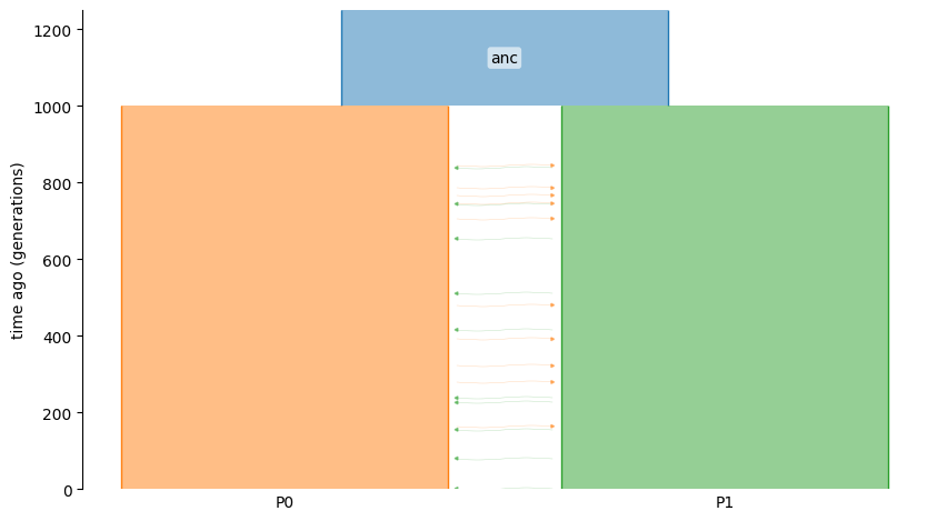
We will simulate a simple isolation-with-migration (IWM) model with two populations.
This uses msprime to build a demography and simulate ancestry/mutations.
import msprime as msp
import demesdraw

demo = msp.Demography()
demo.add_population(initial_size=5000, name="anc")
demo.add_population(initial_size=5000, name="P0")
demo.add_population(initial_size=5000, name="P1")
demo.set_symmetric_migration_rate(populations=("P0", "P1"), rate=0.0001)
demo.add_population_split(time=1000, derived=["P0", "P1"], ancestral="anc")

g = demo.to_demes() # this demes.Graph g will be the input to demestats
demesdraw.tubes(g)
Simulate ancestry and mutations, with 10 diploids from each population:
sample_size = 10
samples = {"P0": sample_size, "P1": sample_size}

anc = msp.sim_ancestry(
    samples=samples,
    demography=demo,
    recombination_rate=1e-8,
    sequence_length=1e8,
    random_seed=12,
)

ts = msp.sim_mutations(anc, rate=1e-8, random_seed=13)
For more details regarding simulation, please refer to msprime.
ICR: Exact and Mean-Field Curves
The ICRCurve and ICRMeanFieldCurve objects are the core components. First, construct the objects by passing in a demes.Graph and a sample size k.
Then, you can use that object to map a set of time points and sampling configuration to the expected ICR curve under a demographic model.
We use a geometric time grid so the plot has more resolution in the recent past.
The lower endpoint is positive because geomspace does not include zero.
import numpy as np
import jax.numpy as jnp
from demestats.icr import ICRCurve, ICRMeanFieldCurve

t = jnp.geomspace(1.0, 5_000.0, 250)
small_ks = [2, 4, 8]
all_ks = [2, 4, 8, 16, 32, 64]

def balanced_samples(k: int) -> dict[str, int]:
    return {"P0": k // 2, "P1": k - k // 2}

def icr_values(curve_out) -> np.ndarray:
    return 1.0 / np.asarray(curve_out["c"])

icr_exact = ICRCurve(demo=g, k=2)
expected_exact = icr_exact(params={}, t=t, num_samples={"P0": 1, "P1": 1})
# you can also call it together with: ICRCurve(demo=g, k=2)(params={}, t=t, num_samples={"P0": 1, "P1": 1})

icr_meanfield = ICRMeanFieldCurve(demo=g, k=2)
expected_meanfield = icr_meanfield(params={}, t=t, num_samples={"P0": 2, "P1": 0})
Note that passing in params={} evaluates the expected ICR under the constructed demographic model g. The sampling configuration must add up to the sample size k used
to initialize the objects. Using k = 2, {"P0": 1, "P1": 1} represents a sampling configuration where one sample comes from population “P0” and the other comes from population “P1”. Similarly, {"P0": 2, "P1": 0} has two samples coming from population “P0”.
When you inspect icr_exact['c'] or icr_exact['log_s'] you obtain the
coalescence hazard c(t) and the log-survival log_s(t).
Compute exact and mean-field curves
For k = 2, 4, 8 we compute both the exact curve and the mean-field
approximation. For larger sample sizes, we only use the mean-field method.
exact_curves = {}
mf_curves = {}

for k in small_ks:
    num_samples = balanced_samples(k)
    exact_curves[k] = ICRCurve(demo, k=k)(t=t, num_samples=num_samples, params={})
    mf_curves[k] = ICRMeanFieldCurve(demo, k=k)(t=t, num_samples=num_samples, params={})

for k in all_ks:
    if k not in mf_curves:
        mf_curves[k] = ICRMeanFieldCurve(demo, k=k)(
            t=t, num_samples=balanced_samples(k), params={}
        )
Exact vs mean-field
The mean-field approximation is already quite close for modest sample sizes in this example.
for k in small_ks:
    exact_icr = icr_values(exact_curves[k])
    mf_icr = icr_values(mf_curves[k])
    rel_err = np.max(np.abs(mf_icr - exact_icr) / np.maximum(exact_icr, 1e-12))
    print(f"k={k:>2}: max relative error = {rel_err:.2%}")
fig, ax = plt.subplots(figsize=(7.0, 4.0))
colors = plt.get_cmap("viridis")(np.linspace(0.15, 0.85, len(small_ks)))

for color, k in zip(colors, small_ks):
    ax.plot(t, icr_values(exact_curves[k]), color=color, lw=2, label=f"exact, k={k}")
    ax.plot(
        t,
        icr_values(mf_curves[k]),
        color=color,
        lw=2,
        linestyle="--",
        label=f"mean-field, k={k}",
    )

ax.axvline(split_time, color="0.6", linestyle=":", lw=1.5, label="split time")
ax.set_xscale("log")
ax.set_yscale("log")
ax.set_xlabel("time")
ax.set_ylabel("ICR(t)")
ax.set_title("ICR: exact vs mean-field")
ax.legend(frameon=False, ncol=2)
fig.tight_layout()
Scaling to larger sample sizes
The exact method becomes expensive quickly as k grows, but the mean-field
approximation remains practical. The next plot extends the sample size up to
k = 64.
fig, ax = plt.subplots(figsize=(7.0, 4.0))
colors = plt.get_cmap("plasma")(np.linspace(0.1, 0.9, len(all_ks)))

for color, k in zip(colors, all_ks):
    ax.plot(t, icr_values(mf_curves[k]), color=color, lw=2, label=f"k={k}")

ax.axvline(split_time, color="0.6", linestyle=":", lw=1.5, label="split time")
ax.set_xscale("log")
ax.set_yscale("log")
ax.set_xlabel("time")
ax.set_ylabel("ICR(t)")
ax.set_title("Mean-field ICR across sample sizes")
ax.legend(frameon=False, ncol=2)
fig.tight_layout()
As k increases, the total coalescence hazard rises because there are more
lineage pairs that can coalesce, so the ICR decreases. For exploratory work on
large samples, ICRMeanFieldCurve is usually the right starting point.
Parameter overrides
To override and evaluate the model at specific parameter settings:
from demestats.event_tree import EventTree

et = EventTree(g)

# Pick variables (by path) from the event tree.
v_split = et.variable_for(("demes", 0, "epochs", 0, "end_time"))
v_mig = et.variable_for(("migrations", 0, "rate"))

# All other non-selected parameters will use the values specified by model g.
# Construct new parameter setting
params = {
    v_split: 1200.0,
    v_mig: 2e-4,
}
The params dict can then be passed into ICRCurve and ICRMeanFieldCurve:
icr_exact = ICRCurve(demo=g, k=2)
expected_exact = icr_exact(params=params, t=t, num_samples={"P0": 1, "P1": 1})

icr_meanfield = ICRMeanFieldCurve(demo=g, k=2)
expected_meanfield = icr_meanfield(params=params, t=t, num_samples={"P0": 2, "P1": 0})
ICR log-likelihood
For likelihood-based inference, use the ICR log-likelihood helper from
demestats.loglik.icr_loglik.
To compute the ICR likelihood:
from demestats.loglik.icr_loglik import icr_loglik

icr_ll = icr_loglik(
    time=t,
    sample_config=[1, 1],
    params=params,
    icr_call=icr_exact,
    deme_names=["P0", "P1"]
)
In order to use JAX’s automatic differentiation, we cannot pass in dictionaries, so we must split a sample configuration {"P0": 1, "P1": 1} into two pieces,
an array of integers sample_config and an array of strings deme_names for the population names. For example, if one wants to use {"P0": 0, "P1": 2} then
sample_config would be [0, 2] and deme_names would be [“P0”, “P1”]. Note that icr_call requires an ICRCurve or ICRMeanFieldCurve object.
Differentiable log-likelihood
Using JAX’s automatic differentiation capabilities via jax.value_and_grad, one can compute the gradient and log-likelihood. Here we
show an example of computing the gradient with respect to the rate of migration from P0 to P1 at 0.0002.
import jax
param_key = frozenset({('migrations', 0, 'rate')})
sample_config=[0, 2]
deme_names = ["P0", "P1"]

@jax.value_and_grad
def ll_at(val):
    params = {param_key: val}
    icr_ll = compute_loglik(
        time=t,
        sample_config=sample_config,
        params=params,
        icr_call=icr_exact,
        deme_names=deme_names
    )
    return icr_ll

val = 0.0002
loglik_value, loglik_grad = ll_at(val)
Parameterization and constraints
demestats automatically generates parameter constraints for a given model via
EventTree and constraints_for. This is part of the ICR workflow because it defines
the feasible parameter space for ICR-based optimization.
from demestats.constr import EventTree, constraints_for

et = EventTree(g)
variables = et.variables

cons = constraints_for(et, *variables)
A_eq, b_eq = cons["eq"]
A_ineq, b_ineq = cons["ineq"]
Please refer to Model Constraints to understand how to modify the constraints to one’s needs.
Putting it together (minimal optimization sketch)
A full optimizer is not shown here, but the typical flow is:
Create a vector for the parameters of interest (subset of
et.variables).Use
constraints_forto get linear constraints.Construct
ICRCurveorICRMeanFieldCurveobject and obtain the expected ICR.Evaluate ICR log-likelihood and optimize.
If you want a complete optimization example, use the notebook at
docs/tutorial_code/icr_optimization.ipynb and refer to icr Optimization.